The Postmortem Airtime Effect
I was busy on a little side project on radio playlists when the news
broke about the death of Dolores O’Riordan, front singer of The
Cranberries. And sure enough, a few hours later I could see The
Cranberries starting to pop up in the playlists.
Their second album No Need to Argue was one of my favourite CD’s as a
teenager, and so I wondered: how many times would they be played? And it
would it all be ‘Zombie’, or would some of their other gems get air time
as well? After seeing the results though, I realized I had no frame of
comparison and ended up scraping a few other artists to compare their
air time before and immediately after passing away.
Scraping the playlist
There is a website that contains playlists for quite a few Belgian radio stations (unfortunately only the Flemish ones). By using this site rather then the radio’s own sites, I could scrape different broadcasting companies with just one function. I did do some random checks to make sure that the playlists were matching though.
First loading the packages needed and checking whether I am allowed to
scrape this site via the robotstxt package.
library(rvest)
library(xml2)
library(tidyverse)
Am i allowed to scrape?
robotstxt::paths_allowed("https://www.relisten.be/playlists/")
# [1] TRUE
I wrote a read_playlist funcion to scrape the data and return
dataframe with 5 columns: station, date, timestamp, artist and title. I
immediately made a second version for the instances where I would need
to iterate this function, called read_playlist_and_sleep which just
adds 5 seconds in between every iteration.
#function to read a playlist, returning a dataframe with timestamp, artist and title of song
read_playlist <- function(radio, date){

  #assemble link
  link <- paste0("https://www.relisten.be/playlists/", radio, "/", date, ".html")

  #playlist info
  html_playlist <- read_html(link) %>%
    html_nodes(css = "#playlist")

  #get time info
  time <- html_playlist %>%
    html_nodes(css = ".media-body > h4 > .pull-right") %>%
    html_text()

  #get title info
  title <- html_playlist %>%
    html_nodes(css = ".media-body > h4 > span") %>%
    html_text()

  #get artist info
  artist <- html_playlist %>%
    html_nodes(css = ".media-body > p > a > span") %>%
    html_text()

    #check for empty pages and return NA if that's the case - otherwise purrr::map will fail later on
  if (length(artist) == 0) {return(NULL)}

  #assembling the dataframe
  playlist <- data.frame(radio, date, time, title, artist, stringsAsFactors = FALSE)
  playlist$date <- lubridate::dmy(playlist$date)
  playlist
}


#adding system sleep to function
read_playlist_and_sleep <- function(radio, date) {
  Sys.sleep(5)
  read_playlist(radio, date)
}
The Cranberries
#SCRAPING FOR THE CRANBERRIES
#making the selection
dates_selection <- c("15-01-2018", "16-01-2018")

radio_selection <- c("radio1", "radio2", "studiobrussel", "mnm",
                     "joefm", "qmusic", "nostalgie", "antwerpen",
                     "clubfm", "familyradio", "radiofg",
                     "topradio", "vbro", "hitfm")


#making all pair combinations
all_pairs <- merge(dates_selection, radio_selection)
colnames(all_pairs) <- c("date", "radio")

#reading the playlists
playlist_TheCranberries <- map2_df(all_pairs$radio, all_pairs$date, read_playlist_and_sleep)
Before doing breakouts I wanted to make sure that no-one had written it
differently, so I so did a str_view just to check that I wouldn’t miss
any instance in my next codes.
str_view(playlist_TheCranberries$artist, "berrie", match=TRUE) only
returned matches on The Cranberries, showing that here are no
upper-lowercases issues, no remixes or featuring artists are present.
The Cranberries were played 36 times over two days - which didn’t sound like that much. More than 10 radio stations, 48 hours…
cranberries
playlist_TheCranberries %>%
filter(artist == "The Cranberries") %>%
summarise(n=n())
# n
# 1 36
So who played their songs?
The rock-indie-pop station Studio Brussels leads the list, followed by
the current affairs Radio1, and the oldies-channel Nostalgie. The hit
radio stations follow the list.
playlist_TheCranberries %>%
  filter(artist == "The Cranberries") %>%
  group_by(radio) %>%
  summarise(n=n()) %>%
  arrange(desc(n)) %>%
  knitr::kable()
| radio | n |
|---|---|
| studiobrussel | 12 |
| nostalgie | 6 |
| radio1 | 6 |
| mnm | 4 |
| qmusic | 4 |
| joefm | 2 |
| radio2 | 2 |
And which songs did they play?
No surprise: Zombie leads the list, but what is left of the teenager
inside of me is a bit sad that so many of their other songs are not in
there. I would have played the supersad No Need to Argue: There’s no
need to argue anymore. I gave all I could, but it left me so sore. …
The lyrics would have fitted!
playlist_TheCranberries %>%
  filter(artist == "The Cranberries") %>%
  group_by(title) %>%
  summarise(n=n()) %>%
  arrange(desc(n)) %>%
  knitr::kable()
| title | n |
|---|---|
| Zombie | 16 |
| Linger | 7 |
| Ode To My Family | 7 |
| Just my imagination | 2 |
| Daffodil Lament | 1 |
| Dreams | 1 |
| Dreams.. | 1 |
| Salvation | 1 |
How does it compare to other artists?
The biggest issue is that I have no frame of reference: is 36 times a lot, or not? France Gall passed away not too long ago, and Tom Petty. I ended up googling for artists who passed away recently, and some slightly longer ago to have some bigger names to compare as well.
As I was about to scrape a bit more, I rewrote what I had done for the Cranberries in a function - but I changed one thing: I also scraped the same two weekdays just a week before the news came as a “pre-death” measure.
read_all_playlists_on_dates <- function(newsdate, artist) {

  #all available radio stations on the Belgian version of the site
  radio_selection <- c("radio1", "radio2", "studiobrussel", "mnm",
                       "joefm", "qmusic", "nostalgie", "antwerpen",
                       "clubfm", "familyradio", "radiofg",
                       "topradio", "vbro", "hitfm")

  #date selection: day of the news and day after, same two days a week before
  newsdate <- dmy(newsdate)
  dates_post <- c(newsdate,  newsdate+1)
  dates_pre <- c(newsdate-7, newsdate-6)


  #making all pair combinations
  all_pairs_post <- merge(format(dates_post, "%d-%m-%Y"), radio_selection)
  all_pairs_pre <- merge(format(dates_pre, "%d-%m-%Y"), radio_selection)


  #map to iterate over all station-date combinations
  playlist_pre <- map2_df(all_pairs_pre$y, all_pairs_pre$x, read_playlist_and_sleep)
  playlist_post <- map2_df(all_pairs_post$y, all_pairs_post$x, read_playlist_and_sleep)


  #adding info and merging into one dataframe
  playlist_post$timing <- "post"
  playlist_pre$timing <- "pre"
  playlist_df <- bind_rows(playlist_post, playlist_pre)
  playlist_df$death <- artist


  #remove any space bars from artist name
  artist0 <- str_replace(artist, " ", "")

  #save to avoid rescraping
  RDS <- paste0("data/playlist_", artist0, ".RDS")
  saveRDS(playlist_df, RDS)

  return(playlist_df)
}
Let the scraping begin! … Or so I thought. I had looked up Leonard
Cohen’s death date in wikipedia, but he was hardly there in the
playlists - which was obviously beyond odd. Turns out that the news of
his death broke a few days after his death.
Additionally there were some oddities driven by timezones, so I
abandoned the wikipedia dates and decided to look up in one of our
biggest newspapers when the news broke in Belgium about every artist and
take that date as a starting point.
#news in paper on 15/01/2018 om 18:22
playlist_TheCranberries <- read_all_playlists_on_dates("15-01-2018", "The Cranberries")

#news in paper on 07/01/2018 om 14:54
playlist_FranceGall <- read_all_playlists_on_dates("7-01-2018", "France Gall")

#news in paper on 25/10/2017 om 17:36
playlist_FatsDomino <- read_all_playlists_on_dates("25-10-2017", "Fats Domino")

#news in paper on 06/12/2017 om 07:28
playlist_JohnnyHallyday <- read_all_playlists_on_dates("06-12-2017", "Johnny Hallyday")

#news in paper on 20/07/2017 om 21:09
playlist_LinkinPark <- read_all_playlists_on_dates("20-07-2017", "Linkin Park")

#news in paper on 03/10/2017 om 06:23
playlist_TomPetty <- read_all_playlists_on_dates("03-10-2017", "Tom Petty")

#news in paper on 11/11/2016 om 09:31
playlist_LeonardCohen <- read_all_playlists_on_dates("11-11-2016", "Leonard Cohen")

#news in paper on 21/04/2016 om 19:19
playlist_Prince <- read_all_playlists_on_dates("21-04-2016", "Prince")

#news in paper on 11/01/2016 om 16:13
playlist_DavidBowie <- read_all_playlists_on_dates("11-01-2016", "David Bowie")
Assembling all the data
I ended up with 9 databases of more than 17000 rows, most of which
contained data I did not need. The next bit of code finds the lines
where the artist who just died (or will die a week later) is played, and
then merges it all together.
One thing I still did manually is the pattern building for each artist.
I like the str_view function for this as you can show the cases where
the pattern matches or where not, to make sure you didn’t capture too
much, nor too few. For instance Johnny Hallyday was sometimes spelled
Johnny Halliday, or there is a “Prince Mohammed” which has nothing to do
with the Prince I was looking for, so I had to keep him out.
#keeping only the rows with the particular artist of interest
find_match <- function(playlist, pattern) {
  match <- grepl(pattern, playlist$artist, ignore.case = TRUE)
  match_df <- playlist[match,]
}

#building input files
input_playlist <- list(playlist_DavidBowie, playlist_FatsDomino, playlist_FranceGall, playlist_JohnnyHallyday, playlist_LeonardCohen,
              playlist_LinkinPark, playlist_Prince, playlist_TheCranberries,
              playlist_TomPetty)

input_pattern <- c("Bowie", "Fats", "France Gall", "Hall[iy]day", "Cohen",
             "Linkin", "Prince [^M]", "Cranberries", "Petty")

#I built by looking manual in case i had something i didn't want:
str_view(playlist_TomPetty$artist, "Petty", match=TRUE)


#combining all matching rows in one dataframe
match_df <- map2_df(input_playlist, input_pattern, find_match)
So who’s the “post mortem air time king/queen”?
summary_table <- match_df %>%
group_by(death, timing) %>%
summarise(n=n()) %>%
spread(timing, n) %>%
mutate(ratio = post/pre) %>%
arrange(desc(post))
summary_table %>%
knitr::kable(digits=0, col.names = c("Artist", "Frequency post",
"Frequency pre", "Ratio post/pre"))
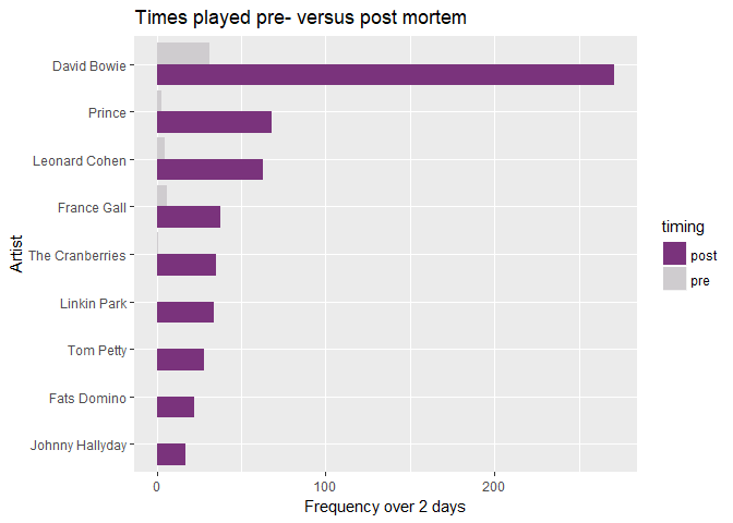
| Artist | Frequency post | Frequency pre | Ratio post/pre |
|---|---|---|---|
| David Bowie | 271 | 31 | 9 |
| Prince | 68 | 3 | 23 |
| Leonard Cohen | 63 | 5 | 13 |
| France Gall | 38 | 6 | 6 |
| The Cranberries | 35 | 1 | 35 |
| Linkin Park | 34 | NA | NA |
| Tom Petty | 28 | NA | NA |
| Fats Domino | 22 | NA | NA |
| Johnny Hallyday | 17 | NA | NA |
Of course: David Bowie! No surprise, although I have to say that I
hadn’t expected such a massive gap between the first two on the list.
After that gap we have Prince and Leonard Cohen, and then with about 30
times played a whole list of artists, including The Cranberries. So
their air time wasn’t too bad after all…
colors <- c("#7a337c", "#CFCCCF")
levels_artists <- summary_table %>%
arrange(post) %>%
pull(death)
ggplot(match_df, aes(x=death, fill=timing)) +
geom_bar(position = position_dodge(preserve = "single"))+
scale_fill_manual(values=colors) +
labs(title ="Times played pre- versus post mortem",
x = "Artist", y = "Frequency over 2 days") +
scale_x_discrete(limits = levels_artists) +
coord_flip()
Which radio’s playlist is most influenced?
radio_summary <- match_df %>%
group_by(radio, timing) %>%
summarise(n=n()) %>%
spread(timing, n) %>%
mutate(ratio = post/pre) %>%
arrange(desc(post))
radio_summary %>%
knitr::kable(digits=0, col.names = c("Radio", "Frequency post",
"Frequency pre", "Ratio post/pre"))
| Radio | Frequency post | Frequency pre | Ratio post/pre |
|---|---|---|---|
| radio1 | 174 | 14 | 12 |
| studiobrussel | 161 | 4 | 40 |
| nostalgie | 69 | 8 | 9 |
| joefm | 39 | 4 | 10 |
| radio2 | 39 | 4 | 10 |
| mnm | 26 | NA | NA |
| qmusic | 23 | NA | NA |
| antwerpen | 21 | 7 | 3 |
| topradio | 6 | NA | NA |
| familyradio | 5 | 2 | 2 |
| clubfm | 4 | 2 | 2 |
| hitfm | 3 | 1 | 3 |
| radiofg | 3 | NA | NA |
| vbro | 3 | NA | NA |
Something else I was curious about: which radio stations change their
playlist most frequently to match what just happened in the world?
Radio 1, the current affairs radio, takes number 1 - not unlogic. A bit
more surprising was Studio Brussels (rock-indie-pop station) following
quite closely. These two were on top for every artist: even artist like
France Gall and Fats Domino who normally would not appear on Studio
Brussels’s playlist were played frequently in the hours after their
death became new.
colors <- c("#7a337c", "#CFCCCF")
levels_radios <- radio_summary %>%
arrange(post) %>%
pull(radio)
ggplot(match_df, aes(x=radio, fill=timing)) +
geom_bar(position = position_dodge(preserve = "single"))+
scale_fill_manual(values=colors) +
labs(title ="Times played pre- versus post mortem",
x = "Radio", y = "Frequency over 2 days") +
scale_x_discrete(limits = levels_radios) +
coord_flip()

Link to github repository with code and data:
https://github.com/suzanbaert/2018_RadioPlaylist